
SQL & Python Pandas Basics
A quick guide on how to use SQL and Pandas for data analysis


This article is part of the Practical Growth Hacks series, where we are going to explore the following topics:
- Coding Skills:
- Essential Growth Metrics & Models:
Customer Activation Strategy
Customer Churn Prediction
Customer LTV Prediction
Booking/Transaction Prediction
AB Testing & Sample Selection
Recommendation Engine
Marketing Mix Model
Market Basket Analysis
Hi fellow growth hackers and data geeks,
If you are coming from the DB setup article and want to learn what functions and commands we are going to use or you just want to refresh your memory, you are at the right place.
As a pre-requisite, you should have setup the database on your local machine; if you haven’t, please visit the previous post.
Alrighty then, let’s start by connecting to our DB and fetching some basic data.
SQL Basics
To connect to our database, we will continue using the Python libraries that we have imported before:
import pandas as pd
import pymysql
Next, we will connect to our database:
host = "localhost"
user = "root" #your username in case you changed
password = "YOUR PASSWORD"
database="analytics" #your database name in case you changed

conn = pymysql.connect(host=host, user=user, password=password, charset='utf8', db=database)
cur = conn.cursor()
If you haven’t encountered any errors, we can proceed to fetch some data. If there was an error, considering the most common reasons, you should double-check whether your MySQL server is running or your password, username, or database name is correct.
Let’s start with our users table. How can we fetch 10 rows of this table so that we can see what kind of data it consists of? The most common SQL command is SELECT. This command helps us get data from the tables we specify. To get the 10 rows, we have to use LIMIT. Limit is quite useful when exploring the database as you ideally shouldn’t fetch the entire rows because it will be costly. Let’s define our query:
query = """
select *
from
users
limit 10
"""
Next, we should execute this query with Python:
cur.execute(query)
df_users = pd.DataFrame(cur.fetchall())
df_users.columns = [desc[0] for desc in cur.description]
Our first line above executes the query while the second creates a Pandas dataframe out of it. By default, your dataframe has no column names. You assign the right column names by executing the third line above.
Now, let’s have a look at the data we received:
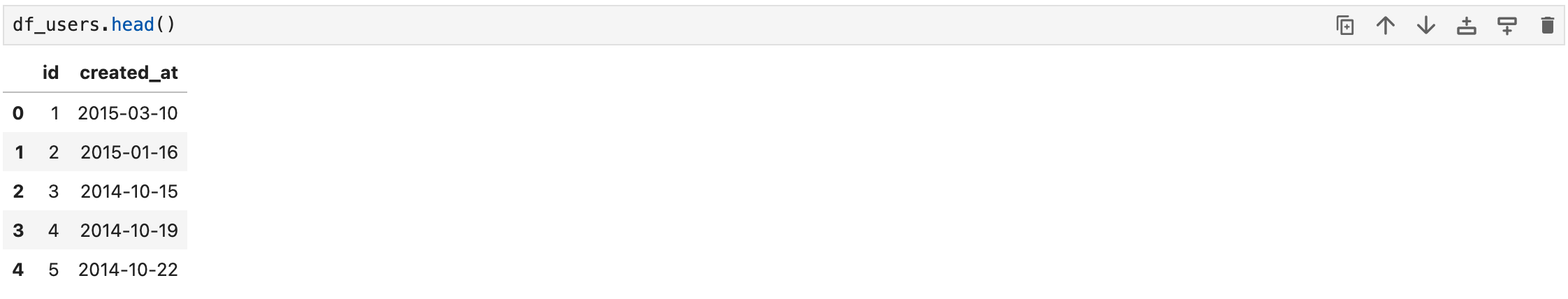
Looking great, we can see the id and created_at columns. Now let’s filter it by the created_at and imagine a scenario in which we’d like to see the users who signed up between March 2015 and April 2016. To do so, we have to use WHERE clause which helps us filter the data based on the conditions we provide:
query = """
select *
from
users
where created_at between '2015-03-01' and '2016-03-31'
"""
As you can see, we have used the ‘‘YYYY-MM-DD’’ date format for filtering the data. But this will not help us in all cases. Sometimes, you have to use some dynamic date filters. Let’s say you want to see the signups in the last 30 days. For this specific example, you have to use:
where created_at > CURDATE() - interval 30 dayIf you go back to the previous example and run the query again:
cur.execute(query)
df_users = pd.DataFrame(cur.fetchall())
df_users.columns = [desc[0] for desc in cur.description]
You will see the updated dataframe by using the .head() function:
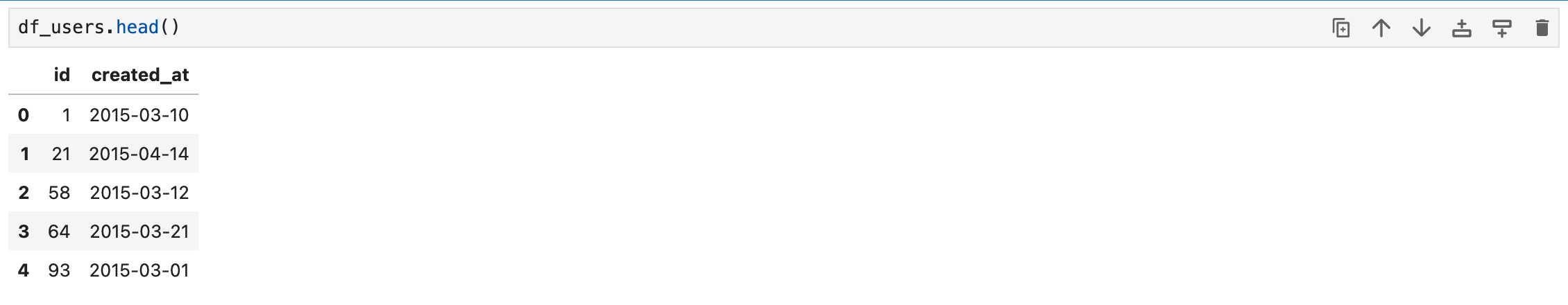
Looking good but the data seems a little bit unstructured. Let’s try to order the data by the signup date. To achieve this, we have to use the ORDER BY clause:
query = """
select *
from
users
where created_at between '2015-03-01' and '2016-03-31'
order by created_at
"""
Let’s run the query and see the results:

I’ve used .head(20) here to show you how it orders in a better way. But as you can easily find out, it has sorted it by older to newer. For doing vice versa:
query = """
select *
from
users
where created_at between '2015-03-01' and '2016-03-31'
order by created_at desc
"""
Adding desc will order the data in a descending order.
Now let’s add a little bit more spice and try to see the number of signups per day. In this case, we will need to count the user ids by using the GROUP BY clause:
query = """
select
date(created_at) as signup_date,
count(distinct id) as user_count
from
users
where created_at between '2015-03-01' and '2016-03-31'
group by 1
order by signup_date desc
"""
There are many new stuff that we have to learn:
1- We have formatted the created_at column by using date(). This helps us convert datetime fields to date.
2- We have used count() to count user ids and we have used distinct to make sure we eliminate any duplicates.
3- Using as enabled us to rename a column. Instead of using created_at, we have used signup_date.
4- Since we have changed the name of the column, we should use this new name for the entire query. That’s why order by created_at changed to signup_date.
5- Lastly, we used the group by clause by adding 1 next to it. This will command MySQL to group by the aggregation by the 1st column, which is signup_date in this case. And group by clause comes before order by in the query syntax.
We are almost there, let’s finish it with JOIN clauses.
Before we go ahead, let’s first check what do we have in the bookings table:
query = """
select *
from
bookings
limit 10
"""
cur.execute(query)
df_bookings = pd.DataFrame(cur.fetchall())
df_bookings.columns = [desc[0] for desc in cur.description]The result will be as follows:
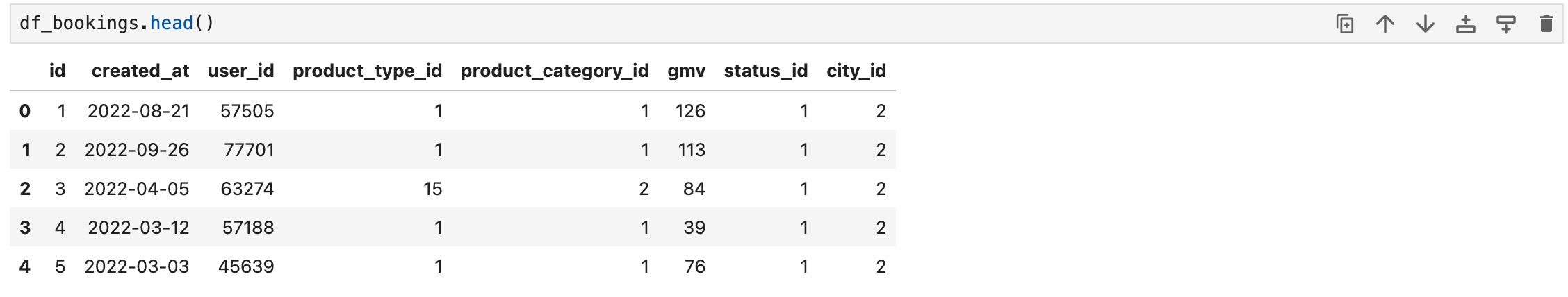
By looking at this number, one question that might come to your mind is: what does city_id represent here? If you are reading this table, you can’t directly understand from which city the booking happened. To answer this question, we have to join this table with the cities table. Let’s explore that table first:
query = """
select *
from
cities
"""
cur.execute(query)
df_cities = pd.DataFrame(cur.fetchall())
df_cities.columns = [desc[0] for desc in cur.description]Our cities table is as easy is below:
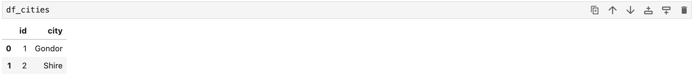
Now let’s merge these both the tables and see from which city each booking is coming:
query = """
select
bookings.*,
cities.city
from
bookings
inner join cities on cities.id = bookings.city_id
limit 20
"""
cur.execute(query)
df_bookings = pd.DataFrame(cur.fetchall())
df_bookings.columns = [desc[0] for desc in cur.description]This is how df_bookings looks now:
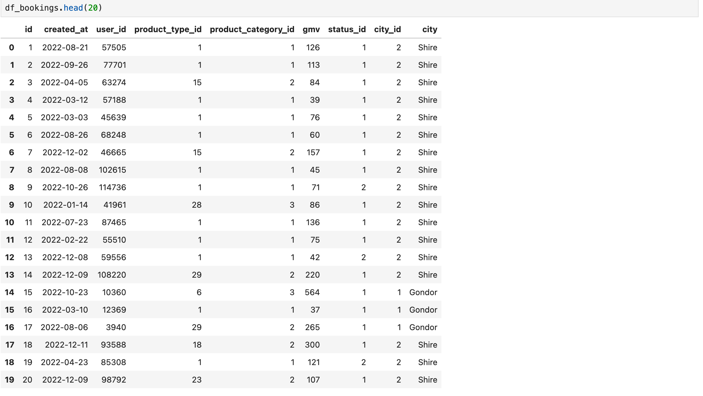
We have a nice little city column added to the query results.
But wait a second, what we have done in the last query:
1- We used something like bookings.*; asterisk here tells MySQL that “return all the columns from the bookings table, while return only the city column from the cities table because I only mentioned cities.city”.
2- For this example, we have used INNER JOIN. Two most important join clauses will be:
Inner Join: This only brings the values that are available for both of the tables. For example, if there weren’t any corresponding value for the bookings’ table city_id = 2 value on the cities table, our query wouldn’t return any booking with city_id = 2. For the same case, if you want to keep your bookings’ table with all its rows and get a NULL under the city column for the bookings for city_id = 2, you should use LEFT JOIN.
Left Join: This join type will help us keep all the values for the first table. But you have to use this join type carefully. If the two tables you want to join have duplicate values, the total duplicates in your result data will multiply. This can end up with long running queries and miscalculations.
There are more exciting stuff that we are going to learn in our journey. I will explain them when we need. But this is already a great start. Let’s look into some Pandas magic now:
Pandas - Python Basics
Up until now, we have used Python for inserting and querying data. Let’s start doing some data manipulation.
First, let’s get the bookings that happened in January 2015:
query = """
select
*
from
bookings
where created_at between '2015-01-01' and '2015-01-31'
"""
cur.execute(query)
df_bookings = pd.DataFrame(cur.fetchall())
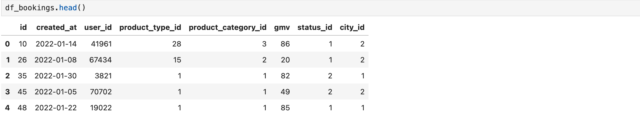
df_bookings.columns = [desc[0] for desc in cur.description]Results:
Now we will start working on df_bookings. Let’s see how many rows and columns we have in it:
df_bookings.shape
As you can see, we have 22439 rows and 8 columns. Before we go into more details, let’s see how we can save our dataframe as a csv file and also read it back from our local machine:
#save as csv
df_bookings.to_csv('bookings.csv',index=False)

#read from csv
df_bookings = pd.read_csv('bookings.csv')
The only small detail that I have to mention here is adding index=False to the to_csv() function. Every Pandas dataframe has an index for each row and we will use it in the future. But we don’t have to save this to the csv file as it doesn’t have any business value for our case.
Let’s continue with how many bookings we have per user. First let’s count them against user id:
df_bookings.groupby('user_id').id.count()If you run the line above, you will see this in your Jupyter Notebook:
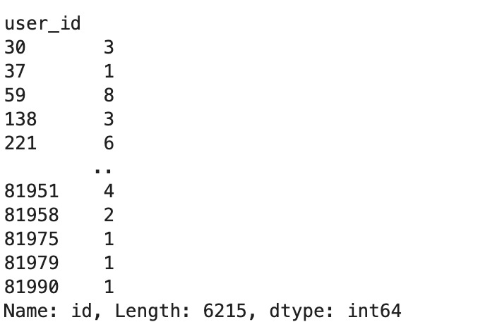
It has calculated it very well, but it is not in a dataframe format. To do that, we have to use the .reset_index() function that converts it to a dataframe by assigning an index.
df_user_bookings = df_bookings.groupby('user_id').id.count().reset_index()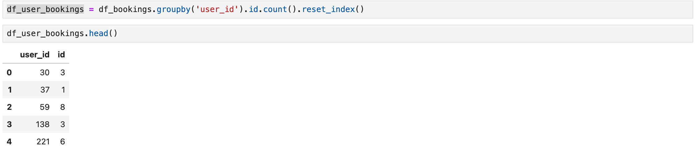
As you can see above, I have also assigned this dataframe to df_user_bookings so that I can refer to that later on.
Now let’s find the average booking per user, but now the user_id and id columns are confusing. First, we will rename our columns and then we will calculate the number we need:
df_user_bookings.columns = ['user_id','booking_count']

df_user_bookings.booking_count.mean()
Jupyter Notebook will print the average booking as you can see above; it is 3.61.
Now, we will do more advanced tricks. We will fetch the booking status table, merge it with the bookings dataframe via Pandas, and then filter it based on these statuses:
query = """
select
*
from
booking_status
"""

cur.execute(query)
df_booking_statuses = pd.DataFrame(cur.fetchall())
df_booking_statuses.columns = [desc[0] for desc in cur.description]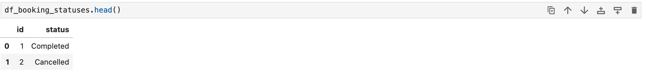
Now let’s merge it with df_bookings table, we will use inner join for this example too:
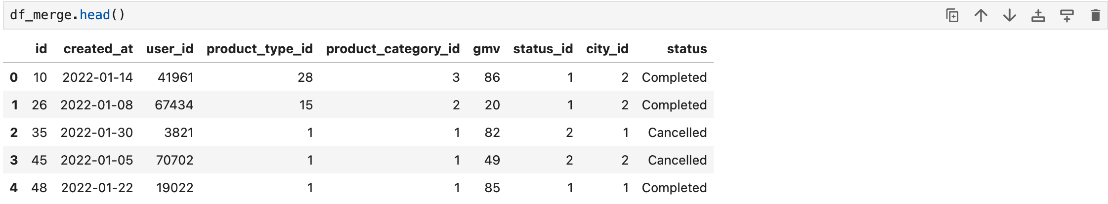
df_booking_statuses.columns = ['status_id','status']

df_merge = pd.merge(df_bookings,df_booking_statuses,on='status_id',how='inner')
Hold on, what happened here?
First we changed the column names of the booking_statuses dataframe.
To merge these two dataframes, we have used pd.merge(). To do that, you have to mention in which column we want to merge these two. In our case, it is the status_id. That’s why we have changed the column names for the booking_statuses dataframe.
And we have selected inner join by using how=’inner’. If I wanted to do a left join, I should have used how=’left’
Let’s see the result:

Now let’s filter it by status and create a new dataframe with only the bookings with status = ‘Completed‘:
df_completed = df_merge[df_merge.status == 'Completed']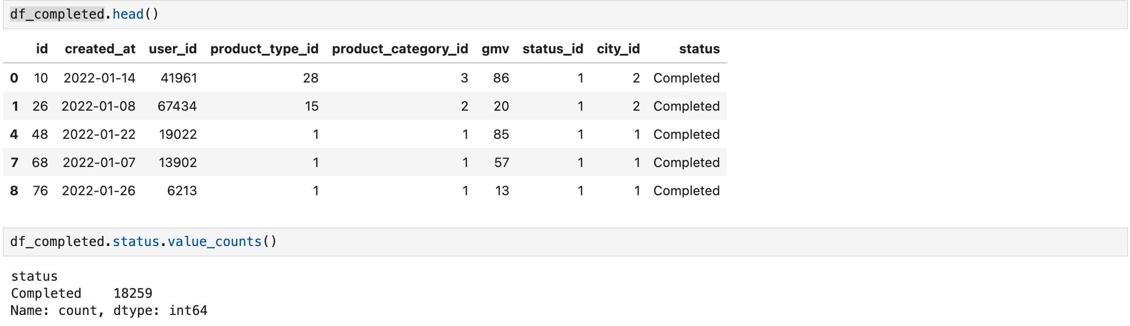
You can see the new df_completed dataframe above. To ensure our status filter has worked, we have used value_counts() after the column we want to check. It only shows completed so our filter has worked properly.
Congratulations! We are going really really fast and learning new tricks. Of course, it is maybe only 5% of it, but this is the fundamentals. Now let’s move on to more sexy ones!
In the next article, we will explore customer metrics (like activation and retention) with pandas and draw some cool charts.
PS. You can find all the Jupyter Notebooks here.